Dataset Browser
This section aims to show you details of the criteria for datasets collection, basic ST analyses performed on our curated ST datasets and tips for navigating them.
1. Criteria for collection
We searched for ST-related articles using keywords of "spatial transcriptomics," "spatial transcriptomic," and "spatial omics" on PubMed, and included ST datasets that contain both gene expression matrices and spatial coordinate information. To ensure the high quality of the database, the ST datasets with both low spot resolution (< 500 spots/cells) and low coverage (< 10,000 detected genes) were discarded. Finally, we collected 100 public ST datasets from humans and mice, with some of these datasets accompanied by imaging data of histological staining. Additionally, we performed Stereo-seq on two sequential coronal sections (10 μm thickness) derived from an embryonic mouse brain at E14.5. These ST data were categorized according to ST technologies, species, strains, organs, tissues, developmental stages and pathological states. This resulted in a compilation of 101 ST datasets comprising 823 sections. All curated ST datasets were uniformly processed using centralized pipelines. We have designed this interface to help you navigate through this catalog. Select the ST data that you are interested in and explore the spatially resolved expression profiles of candidate genes.
2. Dataset attributes
Each dataset comprises the following attributes:
| Attribute | Description |
|---|---|
| ID | Assigned unique ID for each dataset in this web |
| Method | The spatial transcriptomic technology for each dataset |
| Date Published | Date when the data was published |
| Species | Species where the data was derived |
| Strain | Strain of the sample |
| Organ | Organ where the sample was captured |
| Tissue | Tissue where the sample was captured |
| Pathological | True / false meaning whether the sample was pathological |
| Developmental Stage | Developmental stage of the donor |
| Number of Section | Number of technologically sections in each dataset |
| Section ID | Names of sections in this dataset |
| Title | Title of the article where the dataset was published |
| Journal | Journal name of the article where the dataset was published |
| PMID | PMID (pubmed id) of the article where the dataset was published |
3. Data processing
We obtained the gene expression data and spatial location information of 101 sets of spatial transcriptomic data through literature research, some of which contain the image data. A unified python script was used to process the 101 sets of spatial transcriptomic data. The following is the processing procedure:
Basic processing
The scanpy (https://doi.org/10.1186/s13059-017-1382-0) package is primarily used for data preprocessing.
- To begin, we will check if the input data has been normalized or scaled in order to avoid repeating operations.
- The data was then subjected to quality control. We removed the 5% of cells with the lowest total count and the 1% of cells with the highest count, as well as the cells with a mitochondrial RNA expression ratio greater than 25%. For some poor-quality ST datasets, the proportion of mitochondria was relaxed to 30%~50%. At the same time, we eliminated genes that were expressed in fewer than five cells. (In addition to image-based data.)
- The filtered data was then normalized. The first step is to normalize each cell by the total number of all genes, so that after normalization, the total counts of all genes in each cell are the same. The second step is to measure gene expression logarithmically.
- We calculated the high-variable genes after normalizing the data.
- Finally, the dataset is dimension-reduced and clustered. After scaling the data to the unit variance and zero mean, the data was analyzed using principal component analysis, with 50 principal components calculated for each cell. The neighborhood map of the data is then calculated and embedded with UMAP. The Leiden algorithm was used to group the cells (resolution was 0.5, 1, 1.5 and 2, respectively).
Spatial clustering
A spatial region with similar gene expression patterns in a tissue slice is referred to as a spatial domain and has significant biological significance. Therefore, the ability of the spatial transcriptomic to precisely identify such spatial regions is required. STAGATE (https://doi.org/10.1038/s41467-022-29439-6) successfully identifies spatial domains in spatial transcriptomic data using adaptive graph attention auto-encoders.
A spatial neighbor network (SNN) is first built by STAGATE using a predetermined radius. Furthermore, STAGATE uses four layers of graph attention auto-encoders, including two layers of encoders and two layers of decoders, to learn low-dimensional latent representations containing spatial information and gene expression. A normalized expression matrix serves as the autoencoder's input, and the output can be utilized to identify the spatial domain.
This part is mainly handled through the STAGATE_pyG package (https://github.com/QIFEIDKN/STAGATE_pyG) (GPU version of STAGATE).
- We define a parameter scope to estimate the cutoff of constructing a spatial neighbor network in order to better construct a spatial neighbor network. We begin by calculating the distance between spatial transcriptome points along the Y-axis, then averaging the distance to obtain D. The cutoff for constructing the spatial neighbor network is then calculated as D*scope.
- The first step of STAGATE is to build the SNN, which is accomplished through the function "STAGATE_pyG.Cal Spatial Net".
- The second step of STAGATE is to run the main STAGATE method, which is implemented by the "STAGATE.train STAGATE" function.
- The third step of STAGATE is to compute the neighborhood map of the STAGATE output, embed the neighborhood map with UMAP, and then cluster the cells using the Leiden algorithm (resolution of 0.5, 1, 1.5, 2, respectively). This section is handled by a function in the scanpy package.
Marker genes
Finally, the marker genes by eight clustering methods were calculated, including the STAGATE spatial clustering method (four resolutions) and the clustering method based solely on gene expression (four resolutions). This section makes use of the scanpy package's function "tl.rank genes groups".
4. Data visualization
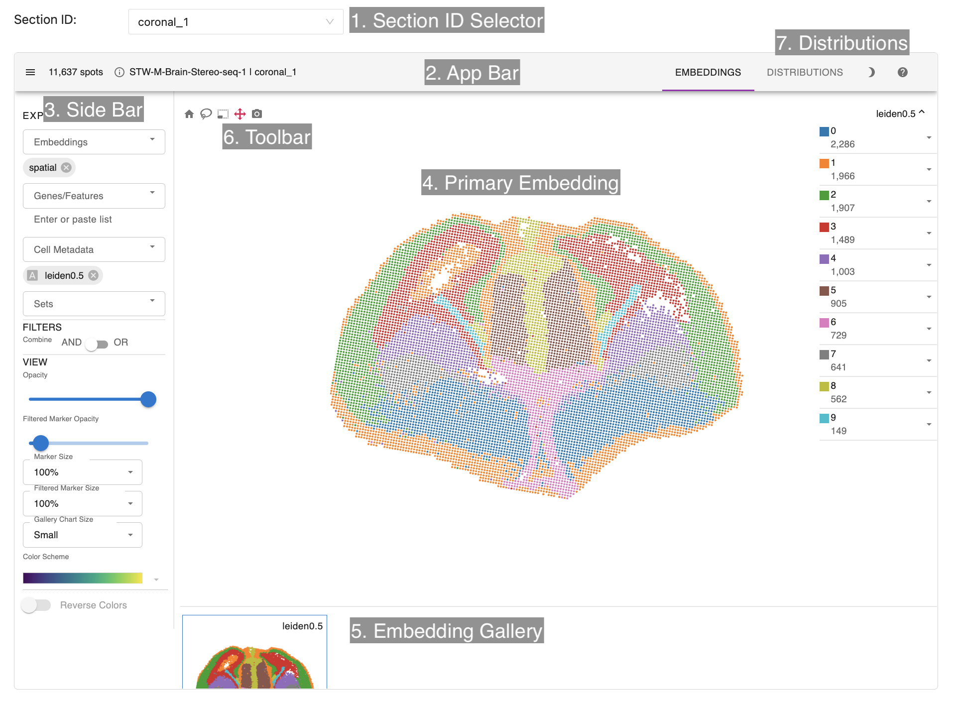
STellaris uses Spatial-Trans-Visual-Tool (https://github.com/Chunfu-Shawn/Spatial-Trans-Visual-Tool) which was developed from Cirrocumulus (https://cirrocumulus.readthedocs.io/en/latest/) for dataset visualization. Cirrocumulus is an interactive visualization tool for large-scale single-cell and spatial transcriptomic data. The data visualization module consists of Sections selector, an app bar, side bar, primary embedding, embedding gallery, toolbar and distribution plots.

- Section ID Selector: allows users to select a section of this datasets to show.
- App Bar: shows the number of cells/spots in your dataset and the number of selected cells. Additionally, it lets you switch between different tabs.
- Side Bar: allows users to select which cell embeddings, genes/features, cell metadata (such as cluster labels) and sets (predefined lists of genes, e.g. cluster markers) to visualize.
- Primary Embedding: allows users to watch and interact with the view of spatial data.
- Embedding Gallery: shows all selected features and embeddings and thus provides a way for comparing attributes and embeddings.
- Toolbar: some tools to select interested spots, download a slice of spatial data and so on.
- Distributions: allows users to explore the differential gene expression across cell clusters with a dot plot, a heat map, or a violin plot.
For more details, please visit https://cirrocumulus.readthedocs.io/en/latest/documentation.html
5. Identification of spatially variable gene
It is critical to analyze spatially variable (SV) genes in the spatial transcriptomic, but the highly variable genes (HVGs) calculated in Scanpy's analysis do not take spatial information into account, so we use SpatialDE (https://doi.org/10.1038/nmeth.4636) methods to compensate.
SpatialDE is a nonlinear and nonparametric method based on Gaussian process regression that can effectively capture differentially expressed genes in space. SpatialDE inputs are raw counts data that have not been normalized, and outputs are the significance of each gene for spatial differential expression.
This section is primarily handled through the SpatialDE package (https://github.com/Teichlab/SpatialDE).
- To begin with, data were preprocessed using the "stabilize" and "regress out" functions from the NaiveDE package (https://github.com/Teichlab/NaiveDE) based on tutorial provided by SpatialDE officials.
- The spatial coordinate data of the spatial transcriptomic data is then extracted.
- The processed gene expression matrix and spatial coordinate information were fed into the "SpatialDE.run" function, and the output result was the p values and q values (Significance after multiple testing) of all genes. Those with q values less than 0.05 were considered to be significant spatially differentially expressed genes and were kept.
6. Description of downloaded file
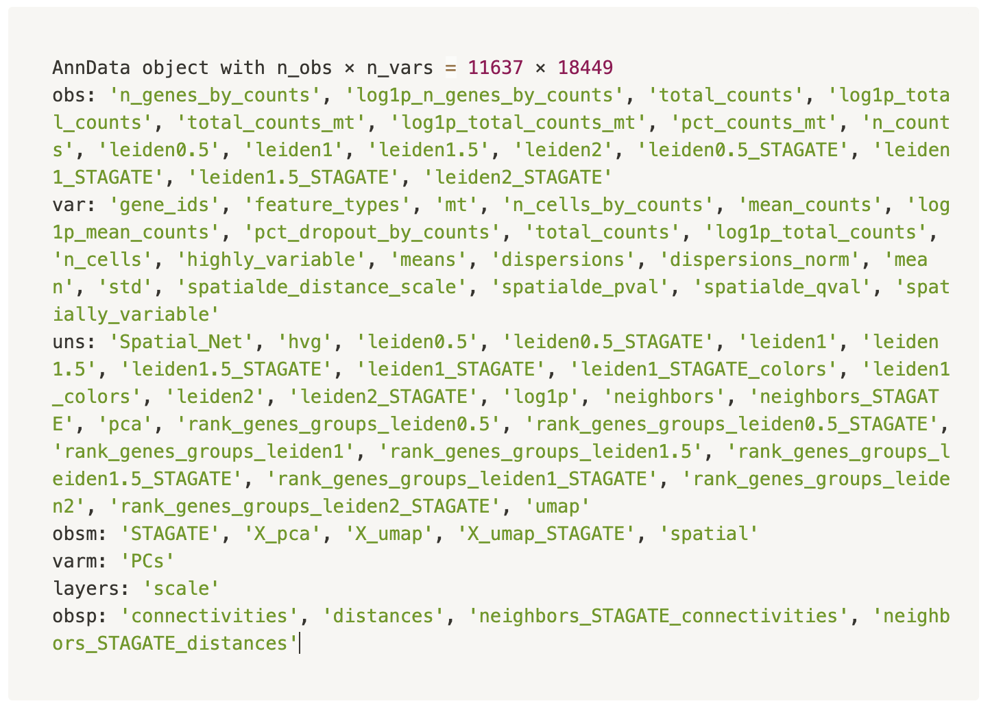
h5ad file is compatible with scanpy/anndata python package, which is highly scalable in python environment. An example h5ad file ready to download is shown below, which contains the results of dimension reduction, traditional clustering, spatial clustering, marker genes of identified clusters and so on.
